Whole-brain Network Measure System by an Integrated Persistent Feature
1. Introduction
Quantitatively characterizing the whole-brain network dynamics is one of the most challenging problems in both structural and functional brain network analyses. Here we propose a novel persistent feature by integrating a prior persistent homology-based topological feature (the zeroth Betti number) and a newly defined connected component aggregation cost feature to model brain networks over all possible scales. The connected component aggregation cost is defined as the summation of subsequent filtration values when a collection of binary brain networks evolves into a fully connected component. We show that the induced topological feature (Integrated Persistent Feature – IPF) follows a monotonically decreasing convergence function and further propose to use its slope as a persistent brain network topological measure. The proposed network feature describes the construction rate from loose components to one fully connected component over a nested filtration graph and thus characterizes information diffusion rate in human brains at the global level. We apply our newly defined measure to study resting-state functional magnetic resonance imaging (rs-fMRI) data from the Alzheimer’s Disease Neuroimaging Initiative (ADNI) and compare our approach with five other widely used graph measures across three parcellation schemes ranging from 90 to 1024 region-of-interests (ROIs). The experimental results show that the new persistent feature shows more statistical power in group difference studies as it is more sensitive to network structure changes. Our proposed measure also exhibits high computation efficiency and a strong robustness to various brain parcellation schemes. Our proposed connected component aggregation cost may empower persistent homology-based brain network dynamics analysis.
2. Software Download and Installation
Download software package here.
This package includes following data and matlab codes.
(1) The detail information of 106 subjects, with 31 AD, 38 MCI, and 37 NC in file subjects.csv. It was acquired from ADNI.
(2) Mean time series of predefined region-of-interests for all 106 subjects with AAL90 atlas in file timecourse_AAL90.mat.
(3) Mean time series of predefined region-of-interests for all 106 subjects with AAL116 atlas in file timecourse_AAL116.mat.
(4) The Brain Connectivity Toolbox (BCT, https://sites.google.com/site/bctnet/) in file BrainConnToolbox.zip.
(5) Our newly defined network measure SIP. Please check the example section to run it.
Installation: This software is designed to run under Matlab 2013a and above. Only the Brain Connectivity Toolboxis required beforehand. Please add BrainConnToolbox path to matlab before running any our program.
3. Data and Methods
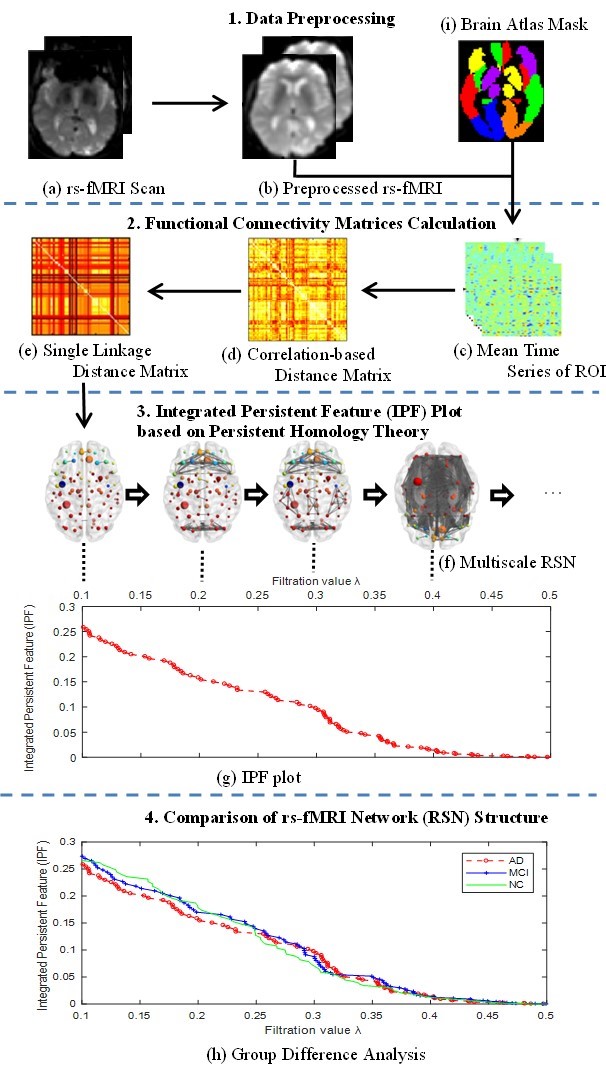
In this study, we define a novel Integrated Persistent Feature (IPF) by combining a prior persistent homology based topological feature (the zeroth Betti number) and newly defined feature (connected component aggregation cost), and propose a corresponding network measure SIP. We compare our measure with another persistent homology-based method, Betti Number Plot (BNP), as well as other four traditional network measures based on graph theory under ADNI resting-state fMRI dataset. The below figure shows the pipeline to compute and discriminate resting-state network (RSN) structure.
3.1 ADNI resting-state fMRI data
Data used in this study were obtained from the Alzheimer’s Disease Neuroimaging Initiative (ADNI) database (http://adni.loni.usc.edu). All participants were scanned using a 3.0 T Philips MRI scanner. The resting state functional MRI (rs-fMRI) were obtained using an echo-planar imaging (EPI) sequence and the parameters included repetition time (TR) = 3000ms, echo time (TE) = 30ms, flip angle = 80◦, number of slices= 48, slice thickness = 3.3 mm, voxel size = 3mm × 3mm × 3mm, voxel matrix = 64 × 64 and total volume = 140. Each participant’s first valid visited rs-fMRI was selected in this study.
3.2 Data Preprocessing
The preprocessing of rs-fMRI data was carried out using SPM8 toolbox, Data Processing Assistant for Resting-State fMRI (DPARSF, http://www.restfmri.net) and Resting-State fMRI Data Analysis Toolkit (REST, http://www.restfmri.net) according to the well-accepted pipelines.
3.3 BNP Method based on Persistent Homology
Hyekyoung Lee, Moo K. Chung, et al. have conducted a range of studies based on persistent homology theory to measure brain network topology features with Betti Number Plot (BNP). Here are some resources related their studies.
https://sites.google.com/site/hkleebrain/home/persistent-homology-2
3.4 Other Measures based on Graph Theory
Numerous studies have confirmed that both structural as well as functional brain networks display the typical features of a small-world organization, modular structure, and highly connected hubs, whose exemplars are the characteristic path length (CPL), modularity, and eigenvector centrality (EC) respectively, thus we compared our work with these three measures as well as network diameter (ND) as the path is obviously important to functional network analysis. We adopted the Brain Connectivity Toolbox (BCT, https://sites.google.com/site/bctnet/) for their implementation.
3.5 Our Proposed SIP Measure
Although BNP shows how the number of connected components changes over different filtration values, the zeroth Betti number only quantifies the invariant feature in a given state, and the estimated information related the future state is not involved. Thus, we introduce connected component aggregation cost to estimate the total cost for completing all subsequent evolutions in a nested filtration graph, and then define an Integrated Persistent feature (IPF) by combining prior persistent homology based topological feature (the zeroth Betti number) and newly introduced feature (connected component aggregation cost).
Furthermore, we define the slope of IPF plot (SIP) as a novel network measure by the linear regression analysis for IPF plot. The number of connected components is getting smaller and the connected component aggregation cost is getting less until all nodes are connected when the IPF is equal to zero, thus the proposed measure SIP may be thought as the information diffusion rate or the convergence speed of arriving to the fully connected component.
4. Examples
4.1 Network Measure with Synthetic data
- In the Matlab command window, type the following command.
>> p= test_synthesis(40,90,100)
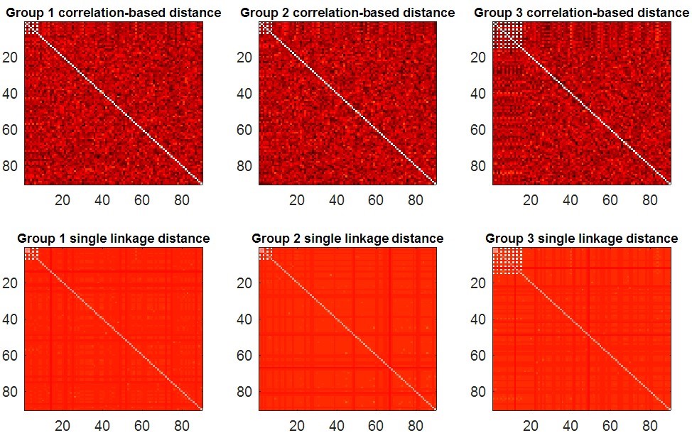
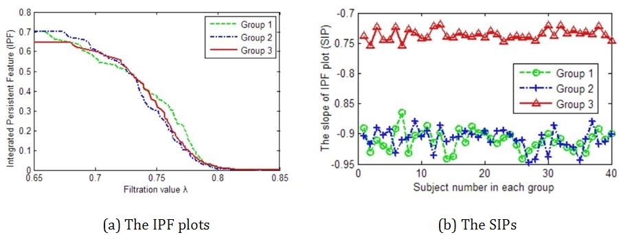
The function synthesizes 3 groups of brain networks with different connected components and then measures these networks by proposed SIP with IPF plot. There are 3 input parameters which denote the sample size in each group, the node size, and the number of time points in each rs-fMRI scan, respectively. The function will display the maps of synthetic data (Fig. 2), and further calculate their IPF (Fig 3. (a)) and SIP (Fig 3. (b)). In the end, the function will return a output parameter which denotes the p-value between simulated networks of group1 vs. group2, and group1 vs. group3.
4.2 Group Difference Analysis with IPF Plot
In the Matlab command window, type the following command.
>> test_brainnetwork(1)
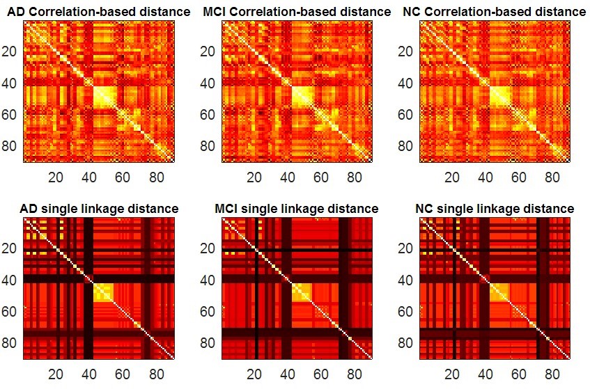
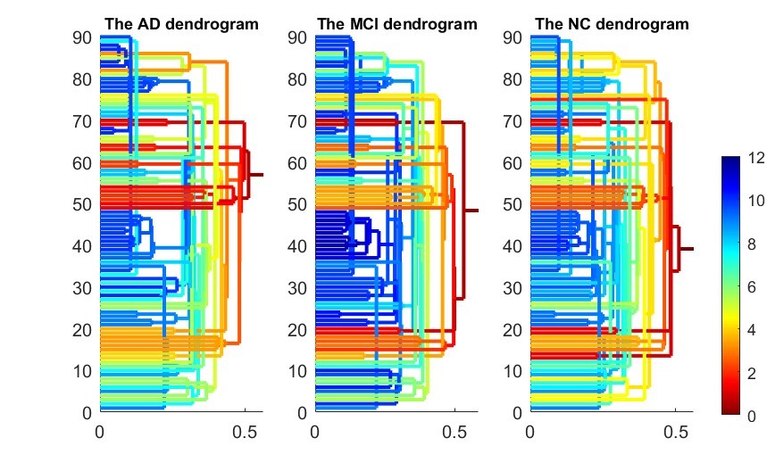
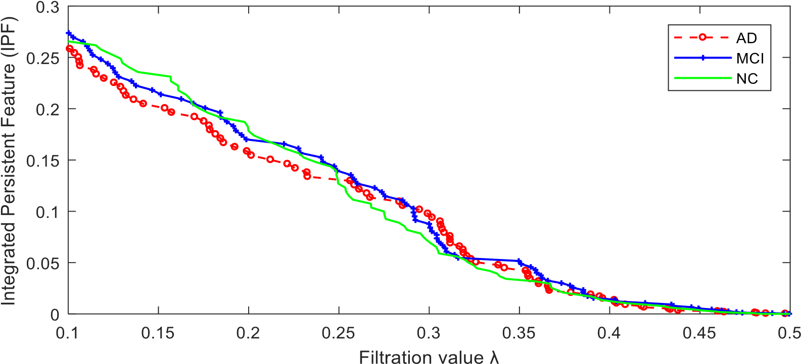
The parameter denotes the number of brain atlas we are going to use. In this example, we use the first atlas, AAL90. This program will display the following figures as results. It produces two functional connectivity matrices (Fig. 4) using SLD method which can be visualized by SLDs (Fig. 5). Then compute and compare different RSN structures by our proposed IPF plot method (Fig. 6). In the end, the function will return output parameters of measure values and their statistical group differences of AD-MCI-NC. The AD, MCI and NC groups show a significant difference (p-value=0.002) with our proposed measure SIP.
